Apheris Co-Folding Application🔗

Welcome to the Apheris Co-Folding Application. This guide will walk you through the steps needed to deploy, configure, and begin using the application in your local or cloud environment.

Overview🔗

The Co-Folding Application allows you to predict the 3D structures of macromolecule complexes with an emphasis on protein–ligand, protein–protein, and antibody–antigen interfaces using OpenFold3 (OF3) and Boltz-2. The affinity prediction capabilities of Boltz-2 are retained.

Key capabilities include:

Quick and convenient deployment to your local cloud or on-prem environment - deploy via pre-built container, AWS CloudFormation Template, or build from source
Model inference (for both OF3 and Boltz-2) with input validation, batch execution programmatically or via a scientist-friendly GUI with built-in visualizations (pLDDT, PAE, structure viewers)

We will soon release additional support for data preparation, benchmarking and fine-tuning.

System Overview🔗

Apheris has created Docker images for its models, built on open-source versions and equipped with an HTTP API wrapper for easy integration with third-party systems.

Models and Requirements🔗

OpenFold3 and Boltz-2 are included in the initial release of the Co-Folding application. Both models are large and can require 25GB disk space or more. These models have been packaged by Apheris as Docker images and can be freely downloaded. The images can be pulled in advance if pulling from our repository is not an option for you environment, please contact us for assistance with this process if needed.

We target the latest release from the respective model providers but for the most up to date information about the model versions see the model description from within the Hub when installing a model.

Recommended Hardware:

Modern GPU with at least 48GB GPU memory (in AWS, the G6e is an example of a cost-effective machine that supports OpenFold3)
At least 300GB of disk space

Architecture🔗

When you select a model for inference in the Apheris Hub, a corresponding Docker container is launched. Initially, only the model container is started, and system resources, including the GPU, are not allocated until a query is submitted. Once a query is processed, the model starts in a subprocess, and the GPU resources are allocated. After the query completes, the GPU is released for future use.

You can submit multiple inference queries at the same time. However, because each query requires full access to the GPU, they are processed sequentially.

When a query is submitted, the input is provided in JSON format as specified in the Running Inference section below, and including any assets uploaded via the "assets" option. These are saved to the input folder specified during the deployment process (see Deployment Guides).

Once inference is complete, the model's predictions and any associated logs are written to the respective output folder and immediately viewable in the UI or accessible by your own external tooling.

Getting Started🔗

Deploy the Apheris Hub🔗

The Co-Folding Application is the first application available within the Apheris Hub and can be easily installed by following our Deployment Guides.

You can install the Hub in a few ways:

After installation, you can access the Apheris Hub from your web browser.

Multiple Sequence Alignment (MSA)🔗

Each model is offered in two flavors, either for using public or private MSA generation.

For public MSA generation, ColabFold is the public MSA server used by default but the specific server the requests are passed through can vary per model.

Note

Any queries submitted using the public-msa versions of models will be sent to the MSA server hosted by, at least, ColabFold. If you do not wish to have your sequences leave your environment, do not use the public MSA versions of the models.

If you use the flavor with the private MSA generation, any traffic to external servers is blocked. So, during inference configuration, you can specify and upload as assets the pre-computed MSA files.
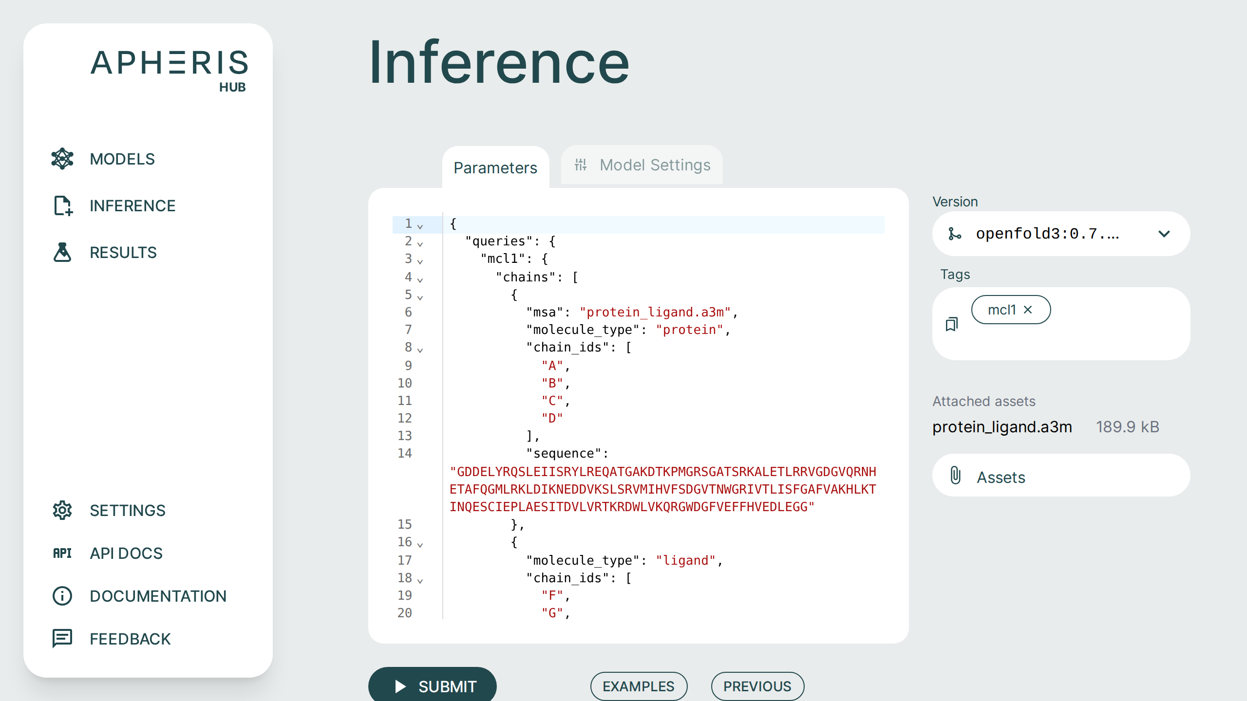
That means you need to generate the .a3m files yourself. For each protein chain in the request, add an extra "msa": "filename.a3m" (input validation will fail if there is no msa field). The *.a3m files should be already located in the input folder, or uploaded through the assets dialog in the inference UI (if they don't exist then input validation will fail).

See the Running Inference section for an example of using your own MSA files for inference.

In future versions we will allow to point to an existing private MSA server that generates these. We from Apheris can also help you set up a private MSA server if you wish, in that case please contact us.

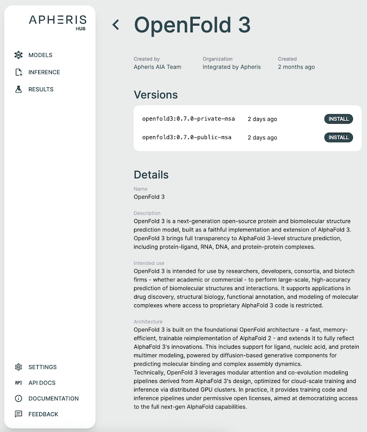
Install Models🔗

The Apheris Hub allows you to download multiple models (currently OpenFold3 and Boltz-2) for the Co-Folding application. These models have been packaged by Apheris (as docker images) and can be freely downloaded. They come with a standardized query payload and can be called via an HTTP API, see Running Inference for more information.

To install a model, navigate to the models screen and select a model and version from the install model list.

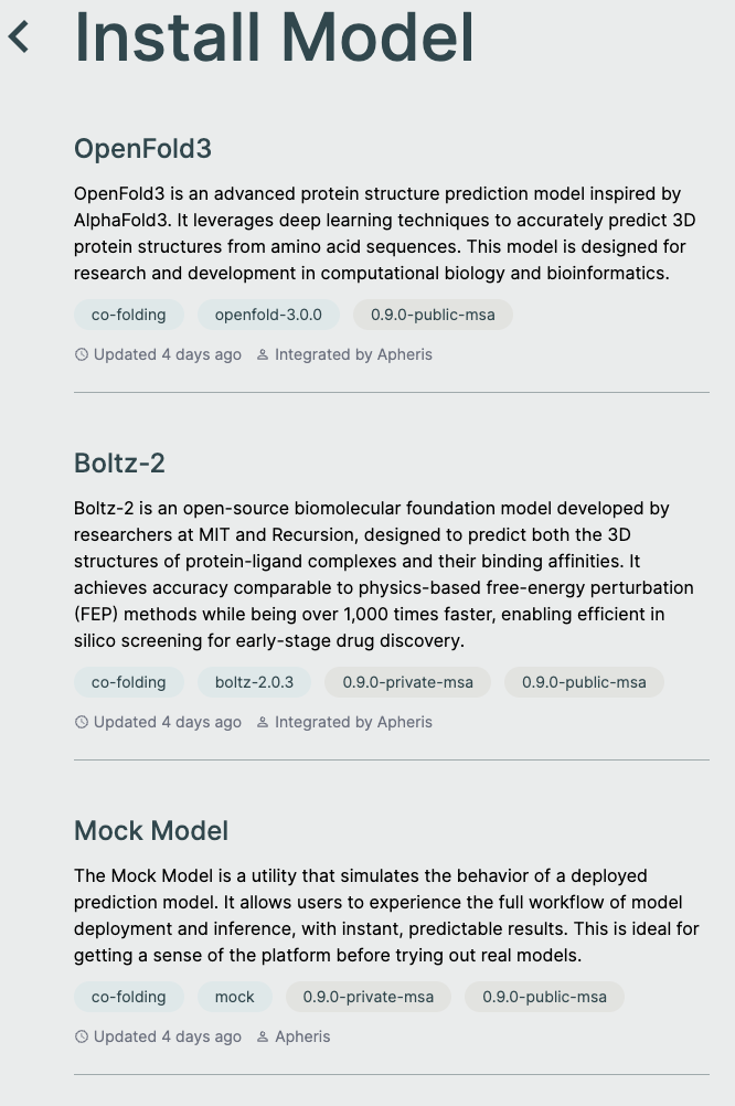
Mock Model🔗

You can also download a Mock Model which is useful for being able to install the Hub locally and test the full end-to-end workflow of the Co-Folding application.

The Mock Model:

Is pulled from the same repository as all other models
Only validates and works with the example queries
Produces results, similar to that of OpenFold3
Results can be visualized and downloaded the same as any other model

Managing Models🔗

Once you have installed a model you can start and stop via the model settings.

The settings page also displays model details including:

MSA server configuration
Container status and uptime
Container port

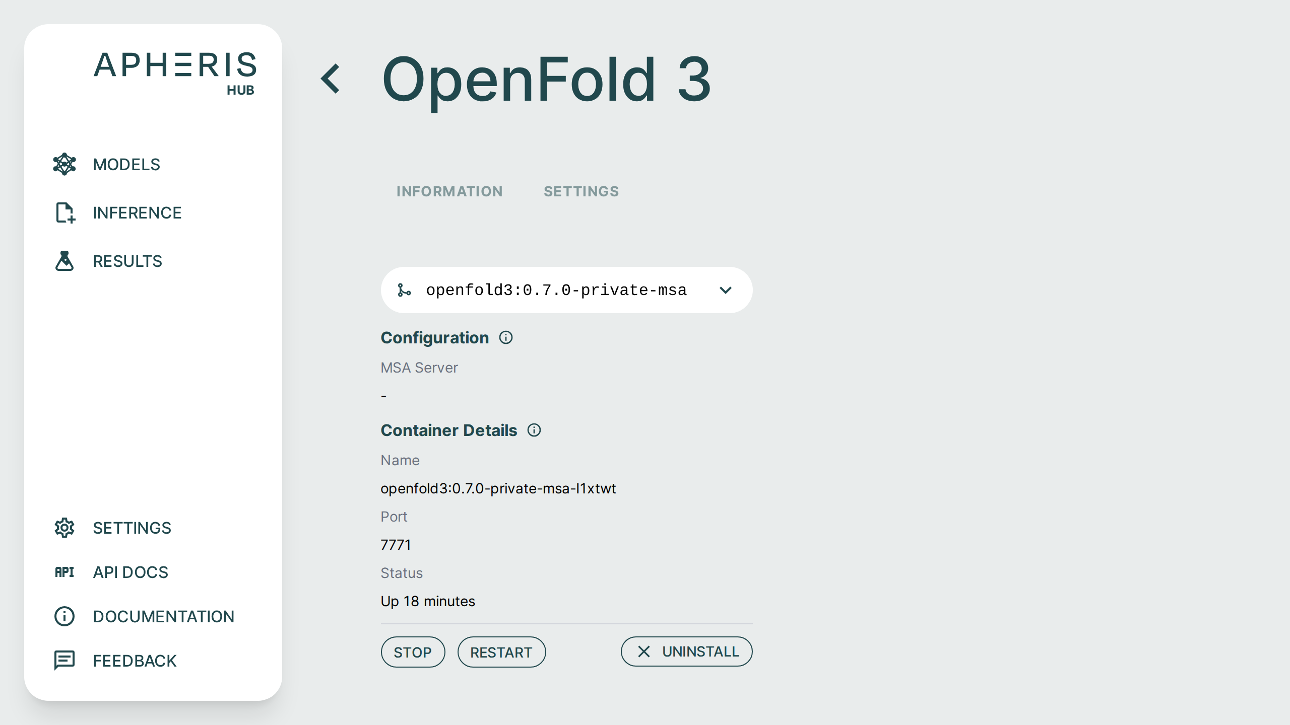
Uninstall Models🔗

In addition to starting and stopping you can uninstall the model from here as well by simply clicking the "Uninstall" button.

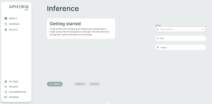
Running Inference🔗

Running inference can be done via the UI or the Hub API. Here, we cover running inference using the UI.

When first clicking on Inference and you only have one model installed, that model container will automatically be started. This happens as the schema validation for the model parameters needs to be first obtained from that model, as this may differ between models and versions.

Multiple Models Installed🔗

If you have multiple models installed, you must first choose which model you'd like to do inference with by selecting the dropdown on the right side.

JSON Editor🔗

The JSON editor offers many convenience features such as syntax highlighting, keyword auto-completion, and data type validation.

Tags🔗

Query names that are supplied in the JSON payload are automatically derived as tags for the job.

Custom Tags🔗

Additionally, you can supply your own tags by typing in the "Tags" field directly. These tags will show connected to the results and can be searched for fast lookups across all queries and results. Custom tags are a great way to distinguish between jobs that might have similar queries.

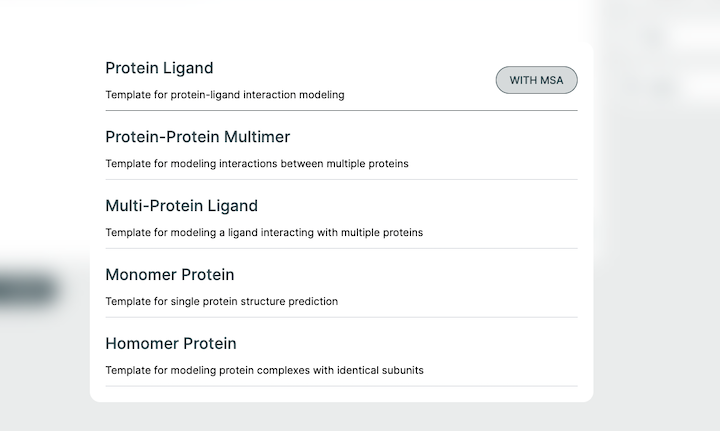
Examples🔗

The Co-Folding application comes with examples to help with getting started. Each of these examples can be run across all models. These can be used as starting templates for your queries or as a simple way to evaluate the full workflow.

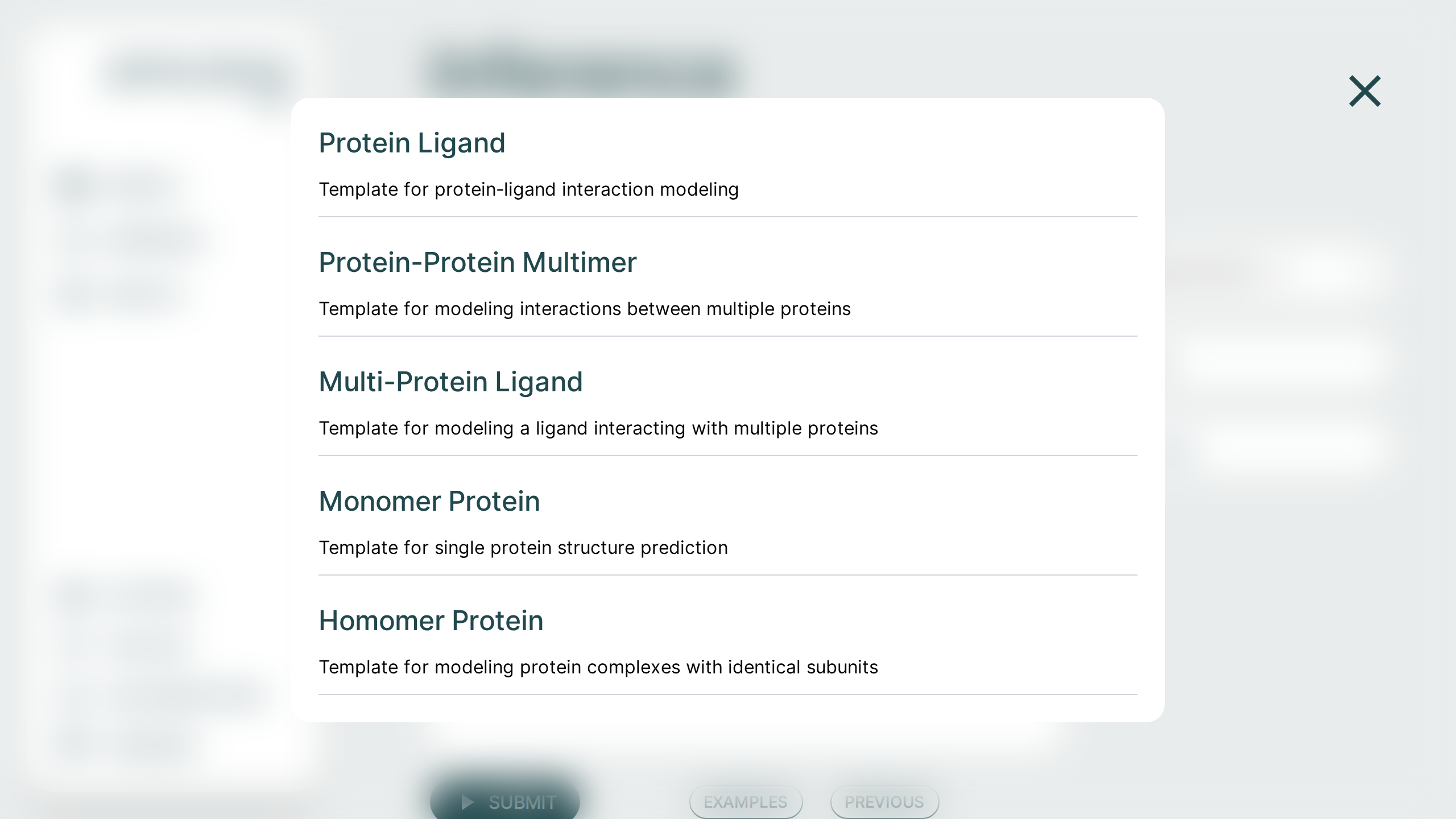
They can each be used with or without an MSA file. The resulting behavior is contingent on the model type you use (private or public).

If you are using a private-msa model, you need to click the "With MSA" that appears when selecting an example.

Assets and MSA files🔗

If your job requires additional assets, such as an MSA file, they can be supplied by clicking the Assets button on the right.

Once you have uploaded your assets they need to be included in your query with the msa field in the JSON editor, as shown below.

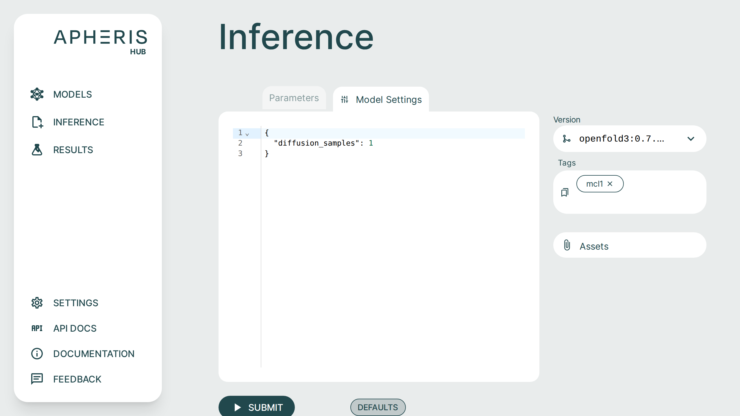
Model Settings🔗

Some models have additional model-specific settings that can be configured such as diffusion samples. These can be changed on the Inference screen by selecting the "Model Settings" tab at the top.

You can click the "Defaults" button to see the available model settings and make changes.

Jobs Management🔗

Whatever you submit in the JSON payload (can be one or multiple queries) is submitted as a single job.

Submitting additional jobs will put those jobs in a queue. The GPU is fully consumed per-job, parallelism and multi-GPU support will come with follow-up releases.

All submitted jobs and results can be viewed on the Results page.

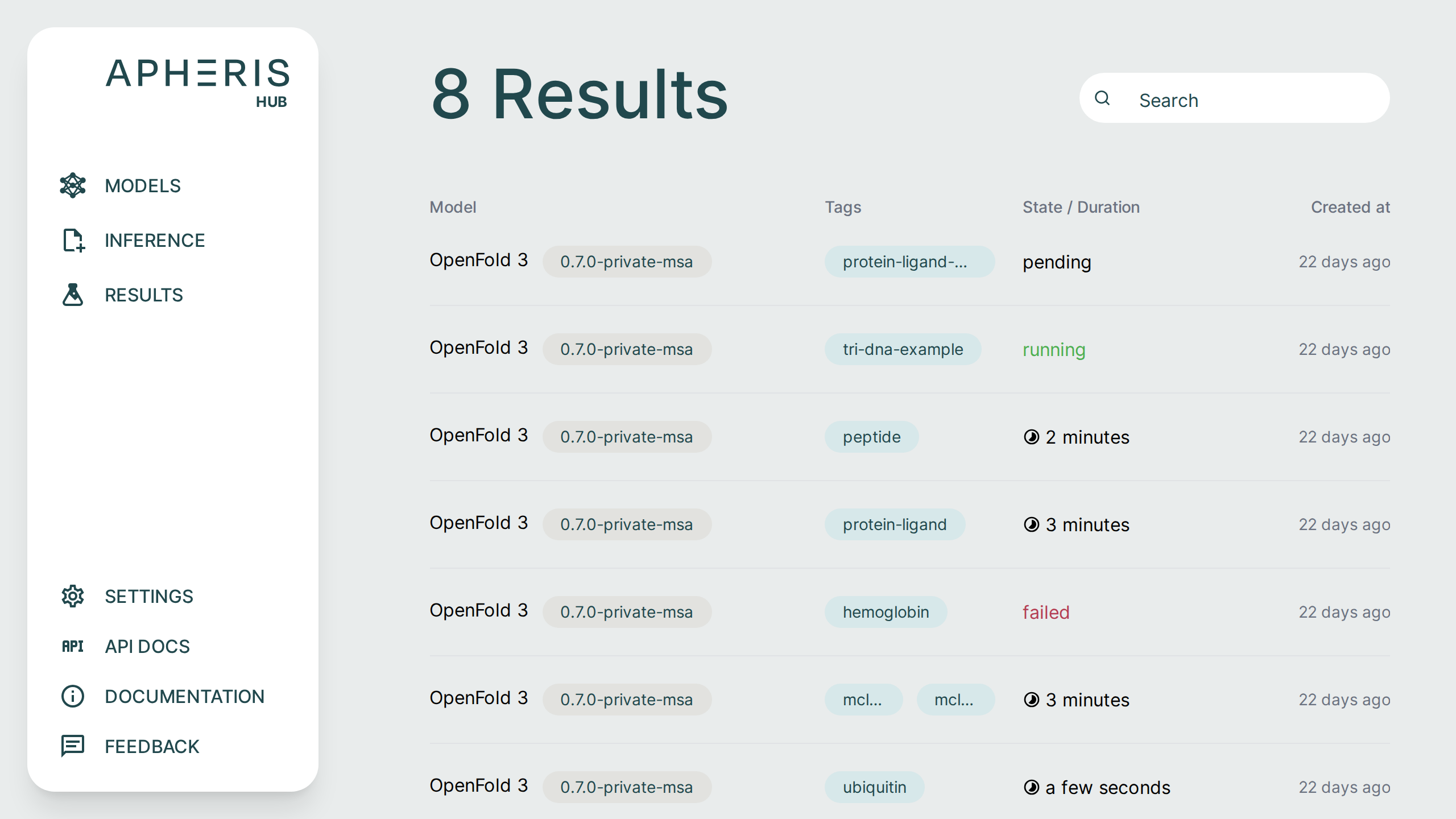
Job Status🔗

Submitted jobs can have a few statuses:

Pending
Running
Failed
Done
- When completed, the status shows the total query runtime.

In addition to the job status you can also see when the job was created, the model and version, as well as any tags associated with the job.

Job Results Deletion🔗

Job results are persisted in the output folder specified when you deployed the Apheris Hub for the first time.

Currently, there is no built-in way to delete these results. Instead, they are managed through the file system. This is an intentional measure to avoid any accidental deletion of valuable insights.

Analyzing Results🔗

The Apheris Co-Folding application comes pre-packaged with specialized analysis tools to support analyzing inference results within the UI.

You can also Download Results by clicking the raw results download button at the top of the results screen.

Each of these visual components serves a specific purpose in interpreting co-folding predictions:

3D viewer: Understand overall fold and domain organization
PAE/PDE: Assess inter-residue or inter-chain confidence
pLDDT plot: Gauge per-residue reliability
Sequence section: Review input-output fidelity and interpret ligand participation

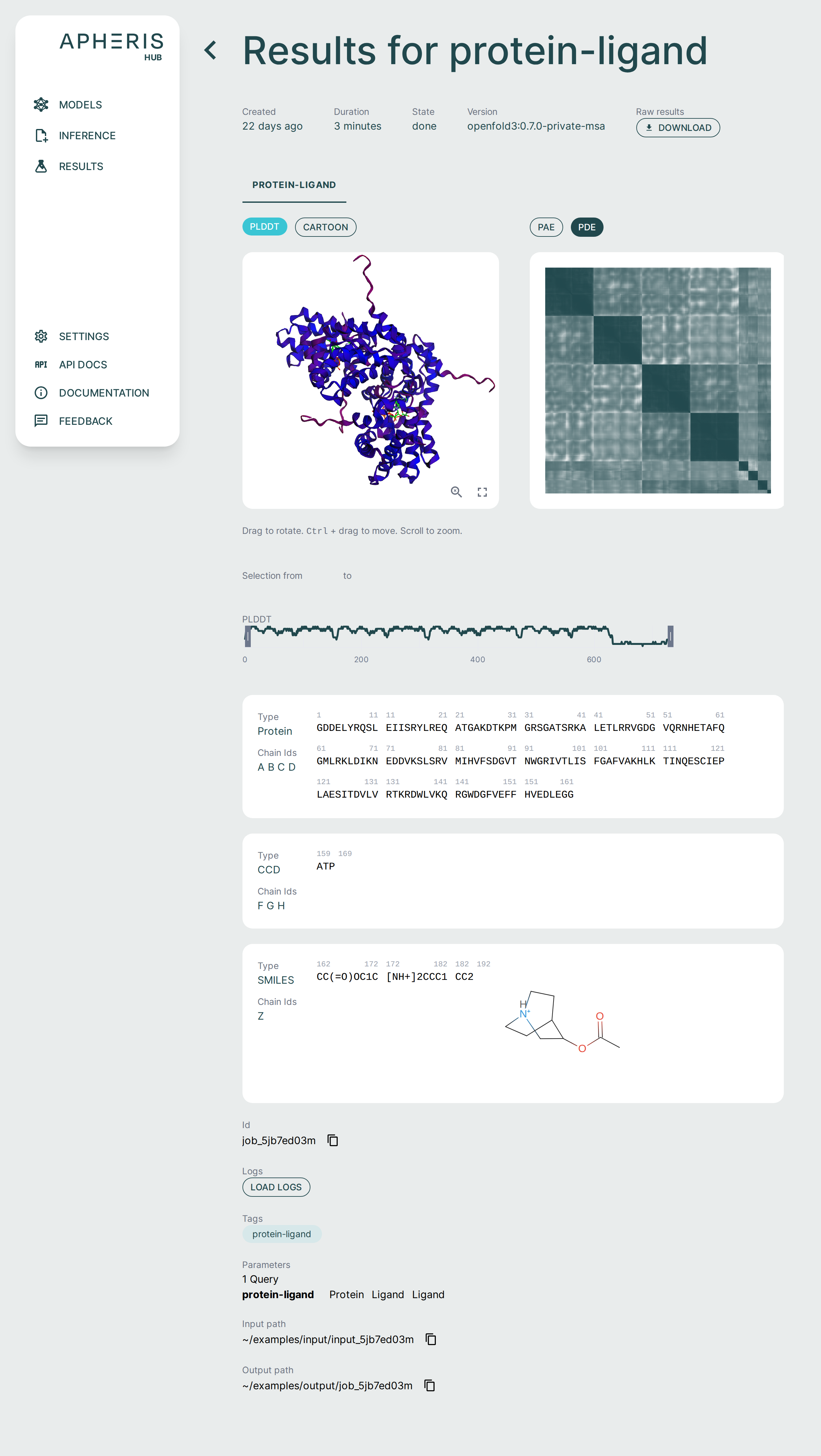
3D Structure Viewer (Left Panel)🔗

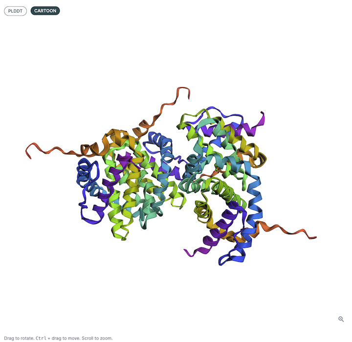
This panel displays the 3D atomic structure of the predicted protein or protein-ligand complex. The cartoon representation emphasizes the secondary structure elements (helices, sheets, loops).

Viewer Color Coding🔗

The structure is colored based on per-residue pLDDT scores, which indicate the model’s confidence in the predicted atomic positions. The scale typically follows:

Blue: Very high confidence (pLDDT > 90)
Green: Confident (70–90)
Yellow/Orange: Low confidence (50–70)
Red: Very low confidence (< 50)

This can be helpful for visualizing local and global structure quality, identifying disordered or uncertain regions, and verifying expected fold topology.

PAE / PDE Matrix (Right Panel)🔗

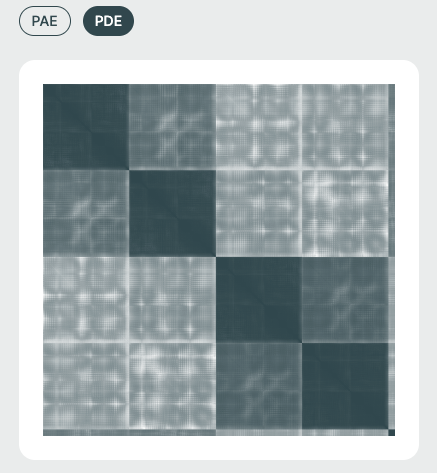
The Pairwise Aligned Error (PAE) or Predicted Distance Error (PDE) matrices visualize the model’s expected error in aligning residue pairs. This is essential for interpreting inter-domain and inter-chain interaction confidence. It is also especially relevant in multi-chain or protein-ligand complexes.

PAE: Captures inter-residue positional uncertainty, which is useful for identifying domain movements and multi-chain relationships.
PDE: (specific to Boltzmann-based models) shows predicted positional deviations, which is useful for uncertainty-aware modeling.

Matrix Color Coding🔗

Darker cells imply lower predicted error (higher confidence), while lighter regions suggest areas of structural uncertainty.

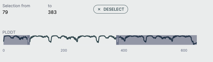
pLDDT Plot🔗

This line graph shows the pLDDT score per residue, providing a quick, global overview of prediction confidence. Ideal for identifying low-confidence loops or disordered regions. Useful for downstream filtering (e.g., in docking, dynamics).

X-axis: Residue index across all chains
Y-axis: pLDDT score (0–100)

Sequence Display🔗

This part is helpful for verifying sequence input/output consistency. Ligand info is key for those focused on drug binding or active site modeling.

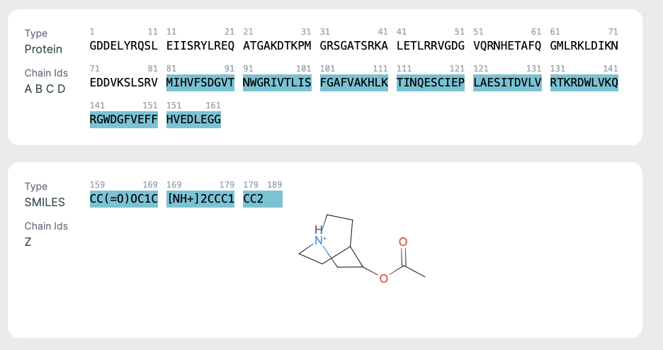
Displays the full amino acid sequence used for the prediction.
Includes chain identifiers (A, B, C, etc.).

Ligand Representation (SMILES)🔗

If a ligand is present (as in co-folding), it is shown in SMILES format along with a 2D molecular rendering.

Troubleshooting🔗

Error: `Model failed to start after upgrade/re-install`🔗

After upgrading or re-installing the Apheris Hub, a model may fail to start if the model server is still running or the port is already in use.

To solve this, shut down the associated running container via Docker.

For example:

$ docker ps
CONTAINER ID   IMAGE                       COMMAND                  CREATED         STATUS         PORTS                                         NAMES
516884069a64   quay.io/apheris/hub:0.1.0   "/application-manage…"   2 minutes ago   Up 2 minutes   127.0.0.1:8080->8080/tcp                      apheris-hub
52652cd32d7f   a34dd83d364a                "python -m uvicorn a…"   47 hours ago    Up 2 seconds   0.0.0.0:7770->8000/tcp, [::]:7770->8000/tcp   mock-0.6.0-public-msa-cKqkmD

Now, stop the running model container and try to start the model again from the Hub UI.

docker stop 52652cd32d7f
52652cd32d7f

Support and Next Steps🔗

To get access to source code, troubleshoot deployment issues, or inquire about connecting to federated environments, please contact: support@apheris.com.