ApherisFold Application🔗
Welcome to the ApherisFold Application. This guide will walk you through the steps needed to deploy, configure, and begin using the application in your local or cloud environment.
Overview🔗
The ApherisFold Application allows you to predict the 3D structures of macromolecule complexes with an emphasis on protein–ligand, protein–protein, and antibody–antigen interfaces using OpenFold3 (OF3), Boltz-2, and Protenix.
Key capabilities include:
- Quick deployment to your local environment, private cloud, or on-premises infrastructure using Docker or Kubernetes
- Model prediction (for OF3, Boltz-2, and Protenix) with input validation, batch execution programmatically or via a scientist-friendly GUI with built-in visualizations (pLDDT, PAE, structure viewers)
- Affinity prediction for protein–ligand complexes, powered by the SandboxAQ affinity head (OF3) and Boltz-2's built-in affinity model
- Benchmarking to evaluate model performance against ground-truth structures with quantitative metrics
- Fine-tuning support for OpenFold3 deployments
System Overview🔗
Apheris has created Docker images for its models, built on open-source versions and equipped with an HTTP API wrapper for easy integration with third-party systems.
Models and Requirements🔗
OpenFold3, Boltz-2, and Protenix are included in the ApherisFold application. These models are large and can require 25GB of disk space or more. These models have been packaged by Apheris as Docker images and can be freely downloaded. The images can be pulled in advance if pulling from our repository is not an option for your environment. Please contact us for assistance with this process if needed.
We target the latest release from the respective model providers. To see which models and versions your deployment is currently using, open the Models page in the Hub (see Models).
Recommended Hardware:
- Modern GPU with at least 48GB GPU memory and CUDA 13+ support (e.g. NVIDIA A100, H100, L40S, RTX 6000 and others). In AWS, the G6e instance is an example of a cost-effective machine that supports OpenFold3.
- At least 300GB of disk space
- Docker environment with Nvidia GPU drivers and the Nvidia Container Toolkit installed
Architecture🔗
The Apheris Hub operates as a coordinator over one or more model services that you deploy alongside it (using the Docker deployment script or Kubernetes Helm chart). Each model runs as its own long-lived HTTP service (for example, a Docker container or Kubernetes Pod) and exposes a standardized prediction API.
The Hub discovers model endpoints from deployment-time configuration (for example, models settings in config.yaml or models.instances in the Helm chart) and routes prediction requests to those endpoints. GPU and CPU resources are managed by your container runtime or cluster scheduler.
In Docker deployments, substantial GPU resources are only allocated while a prediction job is actually running. When a query is submitted, the model service performs the computation and acquires the required GPU resources; once the job has completed, those resources are released so the GPU can be reused for subsequent jobs.
In Kubernetes deployments using the Helm chart, each GPU-backed model runs as a long-lived Pod that requests a full GPU. That Pod retains exclusive access to the requested GPU while it is running, even when no prediction jobs are active. To run multiple GPU-backed models concurrently, use a node with more than one GPU, or deploy only one GPU-backed model at a time per single-GPU node.
You can submit multiple prediction queries at the same time. However, because each query requires full access to the GPU, they are processed sequentially.
With OpenFold3, the first prediction query sent to a freshly started model service will take a bit longer than later queries because optimized GPU kernels are compiled on the fly during that initial request.
When a query is submitted, the input is provided in JSON format as specified in the Running prediction section below, and including any assets uploaded via the "assets" option. These are saved to the input folder specified during the deployment process (see Docker Deployment or Kubernetes Deployment (Helm Chart)).
Once prediction is complete, the model's predictions and any associated logs are written to the respective output folder and immediately viewable in the UI or accessible by your own external tooling.
Getting Started🔗
Deploy the ApherisFold Application🔗
Deploying the ApherisFold Application sets up the Apheris Hub along with enabled models, and configures storage for your data and results. The ApherisFold Application can deploy using either Docker or Kubernetes.
Choose your deployment method:
- Docker Deployment - Deploy using Docker with automated deployment script
- Kubernetes Deployment (Helm Chart) - Deploy to Kubernetes using Helm
After installation, you can access the Apheris Hub from your web browser.
For step-by-step instructions, see the Troubleshooting Guide, which covers common operational problems and provides troubleshooting techniques to help identify, address, or confirm issues.
If you need help or encounter any issues, and the Hub is running, you can generate a Support ZIP archive directly from your web browser (Settings > Support > Download Support ZIP) or via the API. This archive includes system information, Hub configuration, and installed model versions that can help our team better understand your setup. Please email the Support ZIP file, along with a detailed description of your issue, to support@apheris.com.
Models🔗
The Apheris Hub works with multiple models (currently OpenFold3, Boltz-2, and Protenix) for the ApherisFold application. These models have been packaged by Apheris as Docker images and can be deployed in your environment. They come with a standardized query payload and can be called via an HTTP API. See Running Prediction for more information.
Fine-tuning is currently supported for OpenFold3 deployments. Boltz-2 and Protenix support inference only.
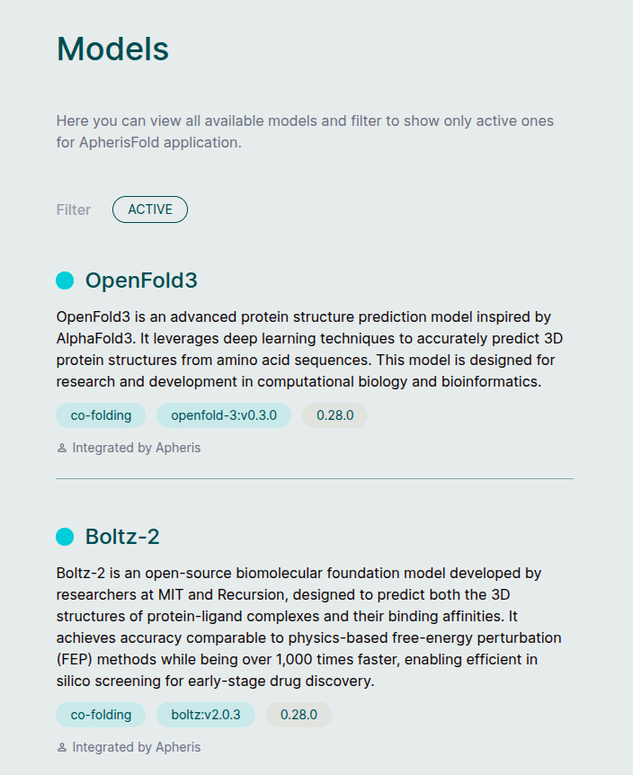
Which models appear in the Hub depends on how your deployment has been configured (for example, via Docker or Kubernetes). Once the Hub is running and can reach the configured model endpoints, the Models screen lists all available models and their discovered versions. Selecting a model opens its details, including descriptions and version metadata.
Mock Model🔗
When enabled, the Mock Model is useful for quickly exercising the full end-to-end ApherisFold workflow.
The Mock Model:
- Is designed to work with the built-in ApherisFold examples (and would fail on unseen inputs)
- Produces example results that are qualitatively similar to OpenFold3 outputs
- Results can be visualized and downloaded the same as any other model
- Does not require GPU resources
To enable the Mock Model, see the Docker Deployment or Kubernetes Deployment (Helm Chart) instructions.
Customizing Model Weights🔗
You can mount custom model weights into your deployment to use custom-trained or fine-tuned models. This is supported for OpenFold3, Boltz-2. Custom weights for Protenix are not currently supported.
Required Files🔗
Each model type expects specific files in the mounted weights directory:
OpenFold3:
of3_ft3_v1.pt(checkpoint file)
Boltz-2:
boltz2_conf.ckpt(confidence checkpoint)boltz2_aff.ckpt(affinity checkpoint)ccd.pkl(coordinate data)mols/(directory containing molecule definitions)
Directory Structure Examples🔗
Your weight files must be organized as follows:
OpenFold3:
weights_mount/
├── additional_weights.json
├── fed/
│   └── of3_ft3_v1.pt
└── fine-tuned/
    └── of3_ft3_v1.pt
Boltz-2:
weights_mount/
├── additional_weights.json
├── custom/
│   ├── boltz2_conf.ckpt
│   ├── boltz2_aff.ckpt
│   ├── ccd.pkl
│   └── mols/
│       ├── ATP.cif
│       ├── GTP.cif
│       └── ...
└── domain-specific/
    ├── boltz2_conf.ckpt
    ├── boltz2_aff.ckpt
    ├── ccd.pkl
    └── mols/
        ├── ATP.cif
        ├── GTP.cif
        └── ...
Configuration Methods🔗
There are two ways to configure custom weights for your models:
Choose One Method
These methods are mutually exclusive. Choose either the configuration file method or the environment variable method, not both. If both are configured, the environment variable (APH_AVAILABLE_WEIGHTS) takes precedence.
Method 1: Using a Configuration File🔗
This method uses a JSON configuration file that you mount into the container. The file path is specified using the APH_WEIGHTS_CONFIG_FILE environment variable.
Deployment-managed weights
For Hub-managed checkpoint deployment, dynamic discovery from the shared weights directory is the primary path. APH_WEIGHTS_CONFIG_FILE and APH_AVAILABLE_WEIGHTS remain supported for backward-compatible manual weights metadata.
When to use:
- You have multiple weight sets with complex configurations
- You want to manage weights configuration separately from deployment configuration
- You need to update weights metadata without redeploying
How it works:
- Create a JSON file with your weights configuration
- Mount the file into the container (via ConfigMap in Kubernetes, or volume mount in Docker)
- Set the
APH_WEIGHTS_CONFIG_FILEenvironment variable to point to the file path inside the container
Method 2: Using an Environment Variable🔗
This method provides the weights configuration directly as a JSON string in the APH_AVAILABLE_WEIGHTS environment variable.
When to use:
- You have a simple configuration with one or two weight sets
- You want all configuration in one place (e.g., Helm values)
- You prefer not to manage separate configuration files
How it works:
- Format your weights configuration as a JSON array
- Set the
APH_AVAILABLE_WEIGHTSenvironment variable with the JSON string - The model reads the configuration directly from the environment
JSON Configuration Format🔗
Regardless of which method you choose, the JSON structure is the same. The configuration should be a JSON object with an available_weights array, where each weight entry contains:
model_type(required): Model identifier -"openfold3"or"boltz2"version(required): Version identifier in semver format (e.g.,"3.0.0-federated"). Models that derive from the OpenFold3-preview architecture are required to start with3.0.0, whereas those from the OpenFold3-release model must be versioned under4.0.0mounted_path(required): Absolute path inside the container where weight files are locateddescription(optional): Human-readable description of the weightsmodel_scope(optional but recommended): Capabilities exposed for that weight.inferencecovers prediction and benchmarking,finetuningcovers fine-tuning jobs, andaffinityadvertises affinity prediction support.model_version_id(optional): Hub model version identifier for compatibility checks - defaults to the current image's version idmodel_version_tag(optional): Hub model version tag for compatibility checks - defaults to the current image's version tag
Please see the example below for OpenFold3 custom weights:
{
    "available_weights": [
        {
            "model_type": "openfold3",
            "version": "3.0.0-federated",
            "description": "OpenFold Federated weights",
            "model_scope": ["inference"],
            "mounted_path": "/weights/openfold3/fed"
        },
        {
            "model_type": "openfold3",
            "version": "3.0.0-fine-tuned",
            "model_version_id": "openfold3:1.2.30",
            "model_version_tag": "1.2.3-openfold3-by-file",
            "description": "OpenFold Fine-Tuned weights",
            "model_scope": ["inference", "finetuning"],
            "mounted_path": "/weights/openfold3/fine-tuned"
        }
    ]
}
Each deployed model instance can expose one or multiple scopes, depending on what model and weights support. Supported scopes are inference for prediction and benchmarking, finetuning for fine-tuning jobs, and affinity for affinity prediction support. In practice, OpenFold3 deployments may expose inference, finetuning, and affinity, Boltz-2 deployments may expose inference and affinity, and Protenix deployments expose inference only. Custom weights can further narrow capabilities per weight through model_scope; omit affinity for weights that do not support affinity prediction.
For clarity, Hub-managed fine-tuned OpenFold3 deployments are currently an exception to the general OpenFold3 capability set above: when you deploy a checkpoint produced by the fine-tuning workflow, the resulting custom weight is structure-only and does not advertise affinity prediction support yet.
The Deployment Examples below illustrate how to set up each method in both Docker and Kubernetes environments. OpenFold3 is used in the examples, but the same principles apply to Boltz-2.
Kubernetes Deployment🔗
This section provides detailed steps for deploying custom weights in a Kubernetes environment using either configuration method.
Important
Ensure your weight files are organized following the structure shown in Required Files and stored in a location accessible by your Kubernetes cluster (e.g., PersistentVolumeClaim backed by EFS, NFS, or hostPath for testing).
Configure Helm Values🔗
Choose your configuration method:
Method 1: Configuration File🔗
Create a ConfigMap with your weights configuration:
apiVersion: v1
kind: ConfigMap
metadata:
  name: openfold3-weights-config
  namespace: apheris-hub
data:
  weights.json: |
    {
      "available_weights": [
        {
          "model_type": "openfold3",
          "version": "3.0.0-federated",
          "description": "OpenFold Federated weights",
          "model_scope": ["inference"],
          "mounted_path": "/weights/openfold3/fed"
        },
        {
          "model_type": "openfold3",
          "version": "3.0.0-fine-tuned",
          "description": "OpenFold Fine-Tuned weights",
          "model_scope": ["inference", "finetuning"],
          "mounted_path": "/weights/openfold3/fine-tuned"
        }
      ]
    }
Apply the ConfigMap:
kubectl apply -f weights-config.yaml
Update your Helm values.yaml:
models:
  instances:
    openfold3:
      deploy:
        image: quay.io/apheris/hub-apps:1.2.3-openfold3-by-file
        env:
          - name: APH_WEIGHTS_CONFIG_FILE
            value: /config/weights.json
        extraVolumes:
          - name: weights-storage
            persistentVolumeClaim:
              claimName: custom-weights-pvc
          - name: weights-config
            configMap:
              name: openfold3-weights-config
        extraVolumeMounts:
          - name: weights-storage
            mountPath: /weights
            readOnly: true
          - name: weights-config
            mountPath: /config
            readOnly: true
Method 2: Environment Variable🔗
Update your Helm values.yaml:
models:
  instances:
    openfold3:
      deploy:
        image: quay.io/apheris/hub-apps:1.2.3-openfold3-by-file
        env:
          - name: APH_AVAILABLE_WEIGHTS
            value: |
              [
                {
                  "model_type": "openfold3",
                  "version": "3.0.0-federated",
                  "description": "OpenFold Federated weights",
                  "model_scope": ["inference"],
                  "mounted_path": "/weights/openfold3/fed"
                },
                {
                  "model_type": "openfold3",
                  "version": "3.0.0-fine-tuned",
                  "description": "OpenFold Fine-Tuned weights",
                  "model_scope": ["inference", "finetuning"],
                  "mounted_path": "/weights/openfold3/fine-tuned"
                }
              ]
        extraVolumes:
          - name: weights-storage
            persistentVolumeClaim:
              claimName: custom-weights-pvc
        extraVolumeMounts:
          - name: weights-storage
            mountPath: /weights
            readOnly: true
JSON Formatting in YAML
When using the environment variable method, ensure your JSON is properly formatted within the YAML value: | block. Each line should be indented consistently.
Deploy with Helm🔗
Upgrade your Helm release with helm upgrade command.
Pod Restart Required
If you're adding custom weights to an existing deployment, you must restart the model pod for changes to take effect, for example for OpenFold3 use:
kubectl rollout restart deployment/hub-openfold3 -n apheris-hub
Verify Configuration🔗
Verify Environment Variables🔗
kubectl exec -n apheris-hub deployment/hub-openfold3 -- env | grep APH_
You should see either APH_WEIGHTS_CONFIG_FILE or APH_AVAILABLE_WEIGHTS set.
Check Volume Mounts🔗
kubectl exec -n apheris-hub deployment/hub-openfold3 -- ls -la /weights/openfold3/
Verify your weight directories are present:
drwxr-xr-x 2 root root 4096 Jan 15 10:00 fed
drwxr-xr-x 2 root root 4096 Jan 15 10:00 fine-tuned
Test Weights Endpoint🔗
Port-forward to the model service:
kubectl port-forward -n apheris-hub svc/hub-openfold3 8000:8000
Query the weights endpoint:
curl http://localhost:8000/weights
Expected response:
{
  "available_weights": [
    ...
    {
      "model_type": "openfold3",
      "version": "3.0.0-federated",
      "description": "OpenFold Federated weights",
      "model_scope": ["inference"],
      "mounted_path": "/weights/openfold3/fed"
    },
    {
      "model_type": "openfold3",
      "version": "3.0.0-fine-tuned",
      "description": "OpenFold Fine-Tuned weights",
      "model_scope": ["inference", "finetuning"],
      "mounted_path": "/weights/openfold3/fine-tuned"
    }
  ]
}
Docker Deployment🔗
This section provides detailed steps for deploying custom weights in a Docker environment using either configuration method.
Important
Ensure your weight files are organized following the structure shown in Required Files and stored in a location accessible from your host machine.
Configuration File🔗
This method uses a separate JSON file for weights configuration, making it ideal for complex setups with multiple weight sets.
Step 1: Prepare your weights directory (Configuration File)🔗
Organize your weight files in weightsDir following the structure in Required Files for your model type.
Step 2: Create a weights configuration file🔗
Create a JSON configuration file (e.g., /path/to/weights/additional_weights.json) that references the directories you created:
OpenFold3 as an Example
This example shows configuration for OpenFold3, but the same approach applies to other supported models (e.g., Boltz-2). Adjust model_type and paths accordingly.
{
    "available_weights": [
        {
          "model_type": "openfold3",
          "version": "3.0.0-federated",
          "description": "OpenFold Federated weights",
          "model_scope": ["inference"],
          "mounted_path": "/weights/openfold3/fed"
        },
        {
          "model_type": "openfold3",
          "version": "3.0.0-fine-tuned",
          "description": "OpenFold Fine-Tuned weights",
          "model_scope": ["inference", "finetuning"],
          "mounted_path": "/weights/openfold3/fine-tuned"
        }
    ]
}
Step 3: Update your configuration (Configuration File)🔗
Update your config.yaml to reference both the weights directory and the configuration file:
models:
  openfold3:
    enabled: true
    weightsDir: "/path/to/weights"
    weightsConfigFile: "/path/to/weights/additional_weights.json"
Inline Environment Variable🔗
This method provides weights configuration directly in the config file as a JSON string, suitable for simpler setups.
Step 1: Prepare your weights directory (Inline Configuration)🔗
Organize your weight files in weightsDir following the structure in Required Files for your model type.
Step 2: Update your configuration (Inline Configuration)🔗
Update your config.yaml by setting the weightsEnv field with your weights configuration as a JSON string:
models:
  openfold3:
    enabled: true
    weightsDir: "/path/to/weights"
    weightsEnv: '[{"model_type":"openfold3","version":"3.0.0-custom","description":"Custom OpenFold3 weights","model_scope":["inference"],"mounted_path":"/weights/openfold3/custom"}]'
Configuration Priority
If both weightsEnv and weightsConfigFile are set, weightsEnv takes precedence.
Deploy🔗
Run the deployment script:
./deploy_apherisfold
The script will:
- Validate your weights configuration (required path settings are present, paths exist, and paths are absolute)
- Mount the weights directory
weightsDirinto the model container at/weightsfolder - Pass the weights configuration to the model via the specified method (file or environment variable)
Verify Docker Deployment🔗
Check configuration🔗
./deploy_apherisfold diagnose
Look for the weights configuration in the output:
models.openfold3.weightsDir:        /path/to/weights
models.openfold3.weightsConfigFile: /path/to/weights/additional_weights.json
Verify container environment🔗
docker exec openfold3 env | grep APH_
You should see either APH_WEIGHTS_CONFIG_FILE or APH_AVAILABLE_WEIGHTS set.
Check mounted weights🔗
docker exec openfold3 ls -la /weights/openfold3/
Test weights endpoint🔗
Access the weights endpoint through the model container's port (check with docker ps):
curl http://localhost:<port>/weights
You should see your custom weights listed in the response.
Using Custom Weights🔗
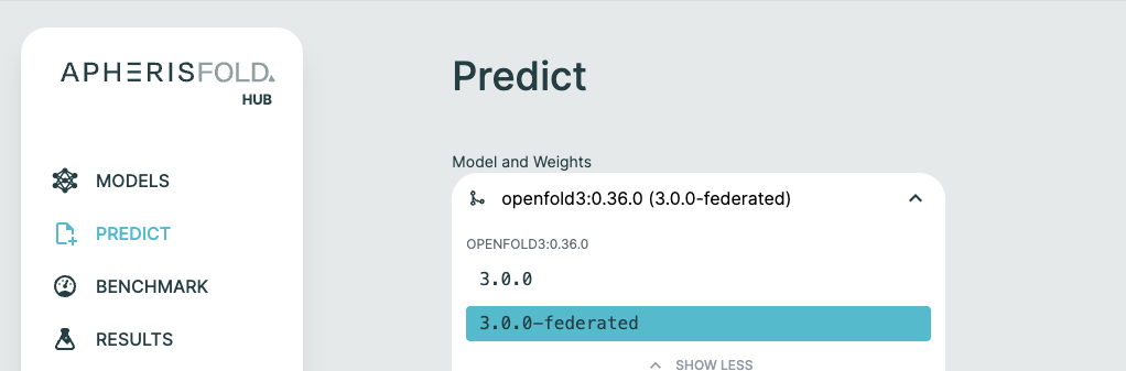
Once configured, custom weights appear in the Hub UI alongside default weights. When creating a prediction:
- Navigate to the Predict page
- Select your model (OpenFold3 or Boltz-2)
- Select your custom weight version from the dropdown
When using the API, specify the custom weight version in your prediction payload:
{
    "id": "1",
    "inputPath": "input/assets",
    "outputPath": "output/results",
    "requestParams": {"queries": {...}},
    "modelName": "openfold3",
    "weightVersion": "3.0.0-federated"
}
Multiple Sequence Alignment (MSA)🔗
MSAs for ApherisFold can be provided either via pre-computed .a3m files, or by using a compatible MSA server implementation. For details on how the Hub generates alignments automatically, see MSA Service.
MSA server definitions are deployment-managed by administrators. In the UI, users can only select one of the configured servers, or disable MSA server usage and upload .a3m files manually.
Supported MSA server types are:
| Provider | Type identifier | Notes |
|---|---|---|
| ColabFold | colabfold |
Supports self-hosted deployments and public servers |
| NVIDIA NIM ColabFold | nvidia-colabfold |
Requires a deployed NVIDIA NIM MSA Search service; see NIM MSA Server Setup |
For configuration instructions, see:
| Platform | Server configuration | Custom headers |
|---|---|---|
| Kubernetes | MSA Server Configuration | MSA Server Headers |
| Docker | MSA Server Configuration | MSA Server Headers |
Important
Any query that uses an MSA server may send protein sequences to that server. If sequences must stay inside your environment, use a self-hosted MSA server or upload pre-computed .a3m files and disable MSA server usage.
Configurable MSA Server🔗
MSA server definitions are configured by administrators at deployment time (Docker config.yaml or Helm values). End users cannot add, edit, or delete MSA servers in the UI.
MSA Request Timeout🔗
MSA request timeout is also deployment-managed (hub.msa.requestTimeout) and applies to backend MSA provider requests.
MSA Usage🔗
The MSA workflow depends on which feature you are using:
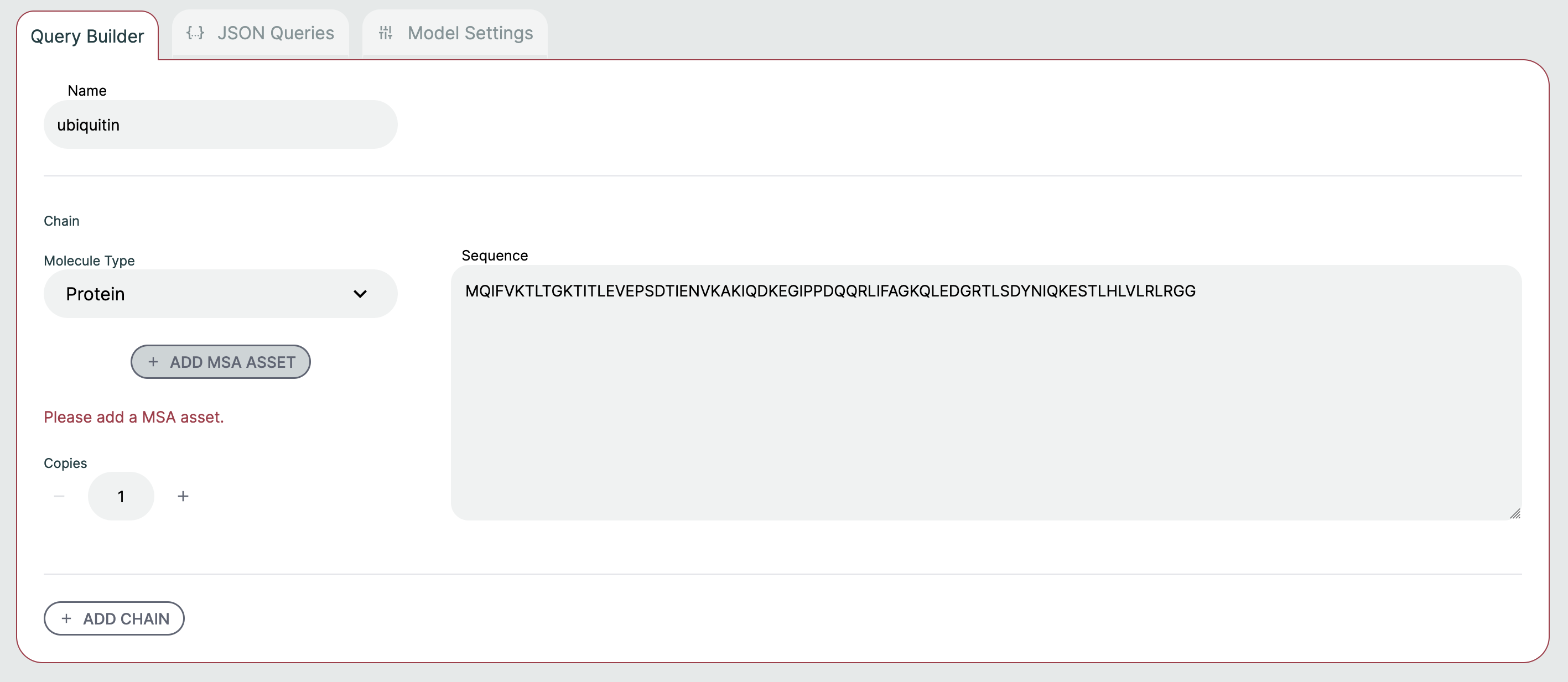
- Prediction: If MSA server usage is disabled, upload
.a3mfiles in the Query Builder. In this mode, no MSA server call is made for that query. For each protein chain, include an"msa": "filename.a3m"field in the query JSON. - Benchmark: If MSA server usage is disabled, attach
.a3mfiles to the benchmark structures before starting the benchmark. - Fine-tuning: Manual
.a3mfiles are attached to dataset structures.
If MSA server usage is enabled in your settings, the Hub creates MSA jobs automatically for chains that do not have uploaded .a3m files. A prediction stays in pending status, a benchmark stays in preparing status, and fine-tuning dataset generation moves the fine-tuning run to preparing until those MSA jobs complete.
If all fine-tuning MSA jobs complete successfully, dataset generation resumes automatically and the fine-tuning run moves to validating. If any MSA job fails, the parent prediction, benchmark, or fine-tuning run fails, and the error reflects the underlying failed MSA job. For benchmarks and fine-tuning runs, the details view keeps that MSA preparation failure visible after reload so you can still inspect the affected query, chain, and error message.
Users can also opt out in Settings and re-enable later by selecting one of the administrator-configured servers.
See also:
- Running Prediction for examples using uploaded MSA files
- Benchmarking for benchmark structure uploads
- MSA Service for prediction, benchmark, and fine-tuning MSA behavior
Affinity Prediction🔗
ApherisFold supports predicting the binding strength between a protein and a small-molecule ligand. The output is a Predicted Affinity value — a pAffinity score (−log₁₀ of the half-maximal binding concentration in µM), where higher values indicate stronger predicted binding. For the currently available models (Boltz2 and the SandboxAQ head for OpenFold 3), this has been trained on a mixture of different assay readouts including pKi/pKd/pIC50/pAC50.
Affinity prediction is available on the Predict page only and applies to protein–ligand queries with a single protein and at least one ligand. It is not available on the Benchmark page.
Supported Models🔗
Affinity prediction is model-specific: each affinity head is trained on embeddings from a particular structural model and cannot be used interchangeably.
| Model | Affinity support | Output |
|---|---|---|
| OpenFold3 Preview 1 (v3.0.0) | SandboxAQ affinity head | Single Predicted Affinity value |
| Boltz-2 | Built-in affinity model | Predicted Affinity ±delta and Binding Probability ±delta |
| Protenix | Not supported | — |
Note
Affinity prediction is only available for OpenFold3 weights that advertise the affinity scope. Hub-managed fine-tuned OpenFold3 checkpoints do not carry over affinity support. See Deploying Fine-Tuned Checkpoints for details.
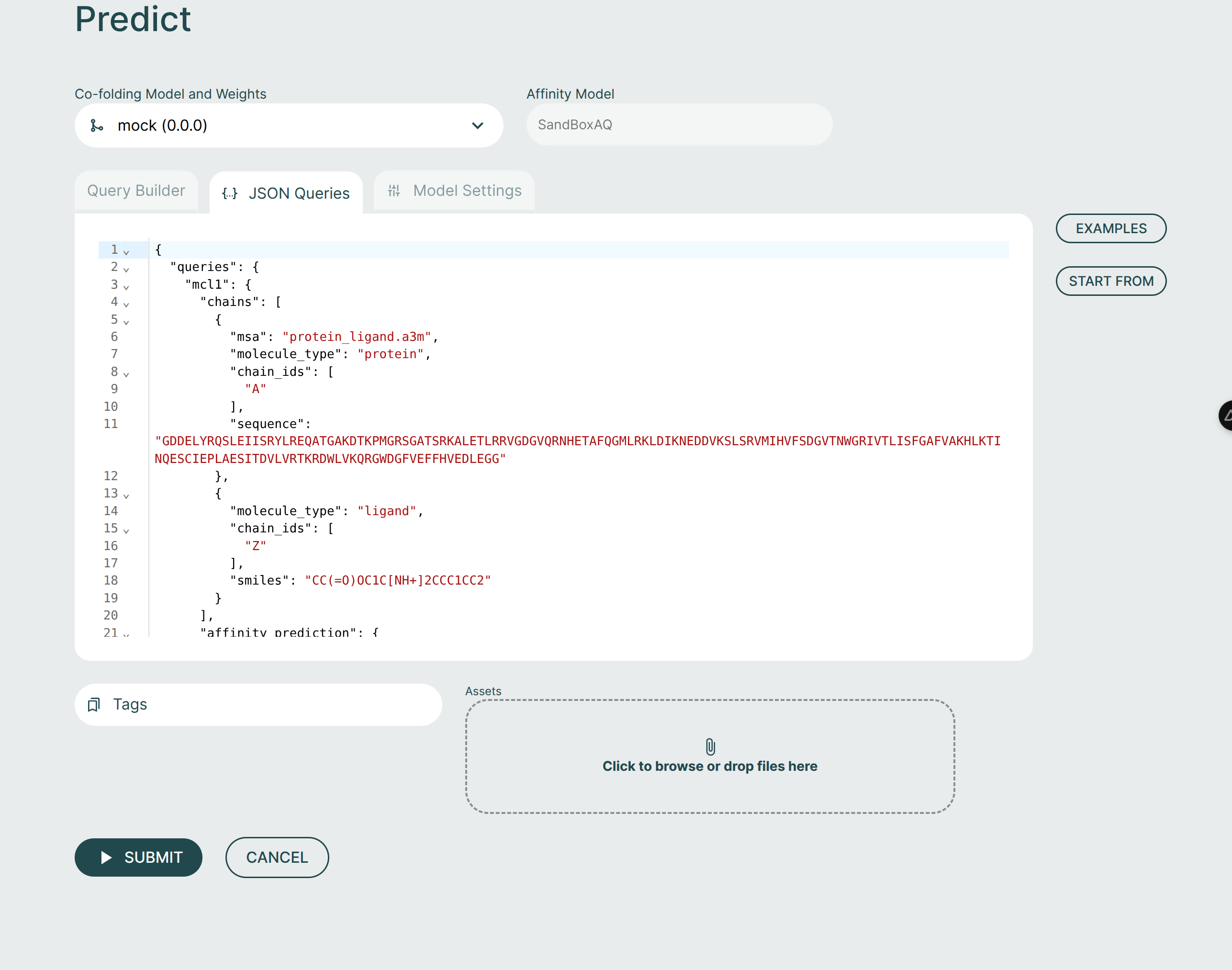
Enabling Affinity Prediction🔗
When you select a co-folding model and weights that support affinity prediction, an Affinity enabled pill appears in the model selection dropdown. No additional configuration is needed — affinity runs automatically alongside structure prediction for eligible queries.
If the selected weights do not support affinity, no pill is shown and affinity prediction is not performed.
Chain Selection🔗
How the protein and ligand chains are selected for affinity depends on your query composition:
- 1 protein + 1 ligand: Affinity is calculated automatically with no additional input required.
- 1 protein + multiple ligands: A radio button appears on each ligand chain. Select the ligand to calculate affinity for. The first ligand is selected by default; only one ligand can be selected at a time.
Note
Affinity chain selection controls are only shown when at least one protein and at least one ligand are present in the query. Queries without a protein–ligand pair (e.g. protein-only or ligand-only) do not display affinity options.
Affinity Results🔗
When affinity prediction runs successfully, the results are surfaced in several places:
- Results table: A Predicted Affinity column appears next to each query's structural metrics.
- Chains section: The Predicted Affinity value is shown alongside the corresponding ligand chain.
- Downloaded metrics file: Affinity values are included in the downloadable results.
For Boltz-2, the results table includes two additional columns: Predicted Affinity ±delta and Binding Probability ±delta. The binding probability is a 0–1 score indicating whether the ligand is predicted to bind at all.
For OpenFold3, a single Predicted Affinity value is returned with no delta.
Caveats🔗
- A high Predicted Affinity score does not guarantee a correct binding pose. The affinity head uses structural embeddings as input and is not a direct proxy for pose quality.
- Prediction quality is best for systems similar to the model's training distribution (PDB-like structures). Confidence decreases for out-of-distribution inputs.
- Affinity fine-tuning to improve predictions for your specific chemical series is planned for a future release.
Running Prediction🔗
Running prediction can be done via the UI or the Hub API. Here, we cover running prediction using the UI.
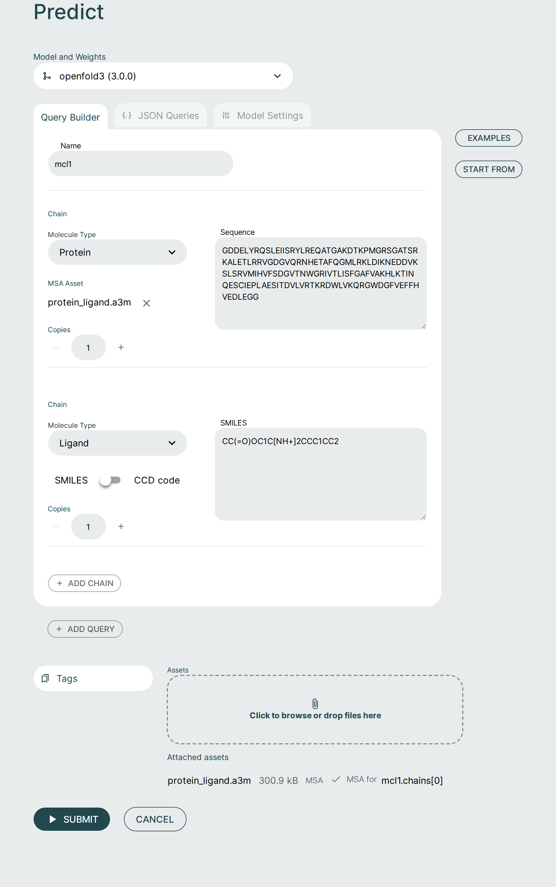
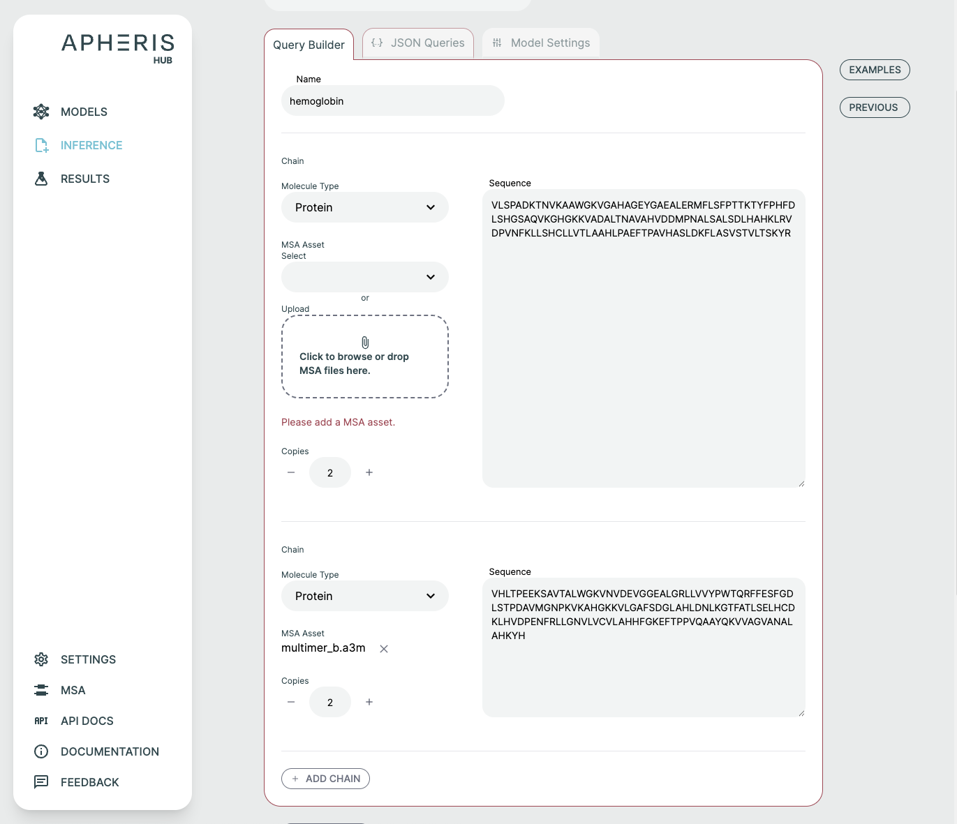
Query Builder🔗
It is possible to form a prediction query using the graphical Query Builder and the JSON Queries Editor.
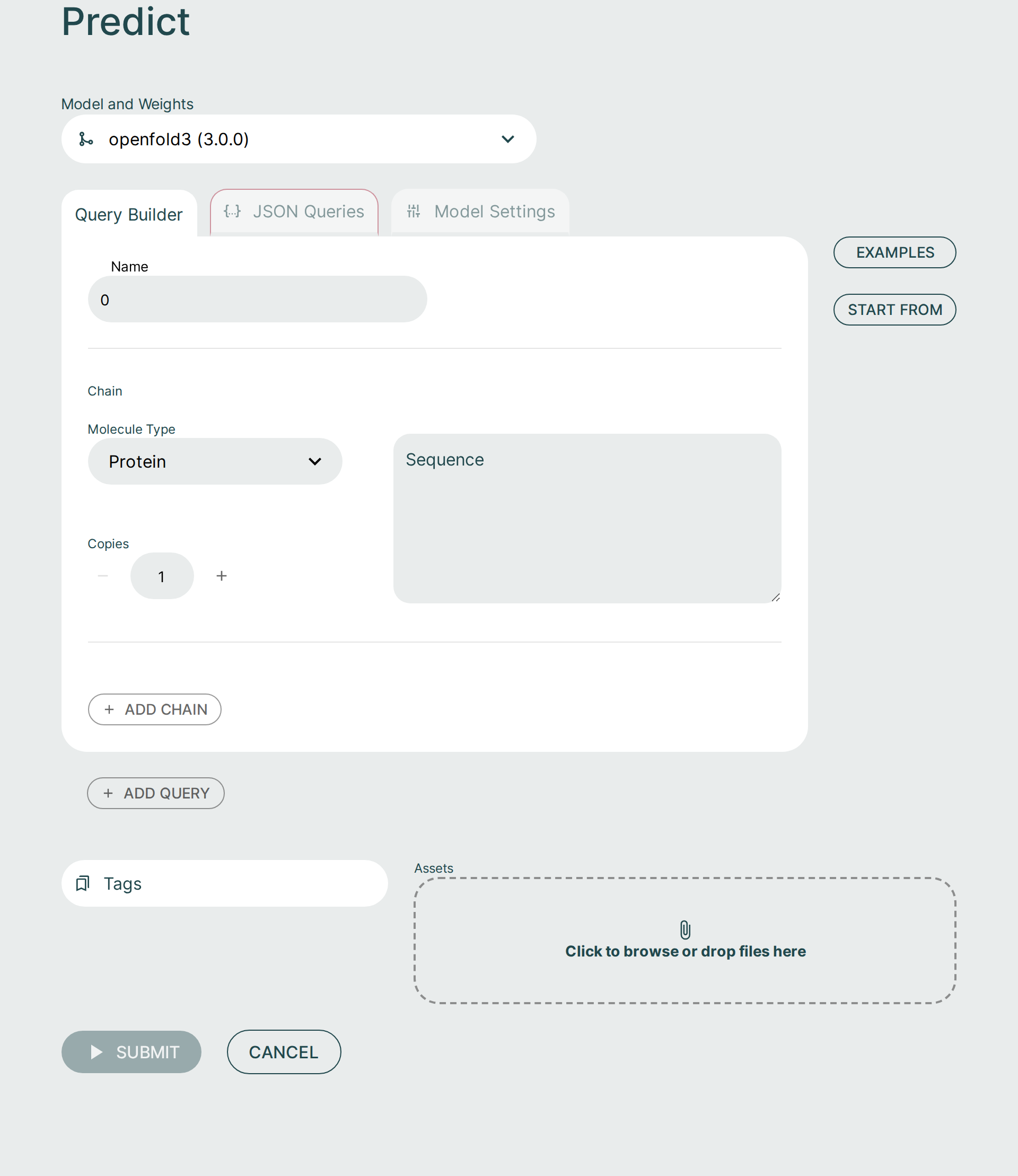
You can add to and adjust the query to fit your needs. It is possible to make changes as well as add additional components or chains to the query.
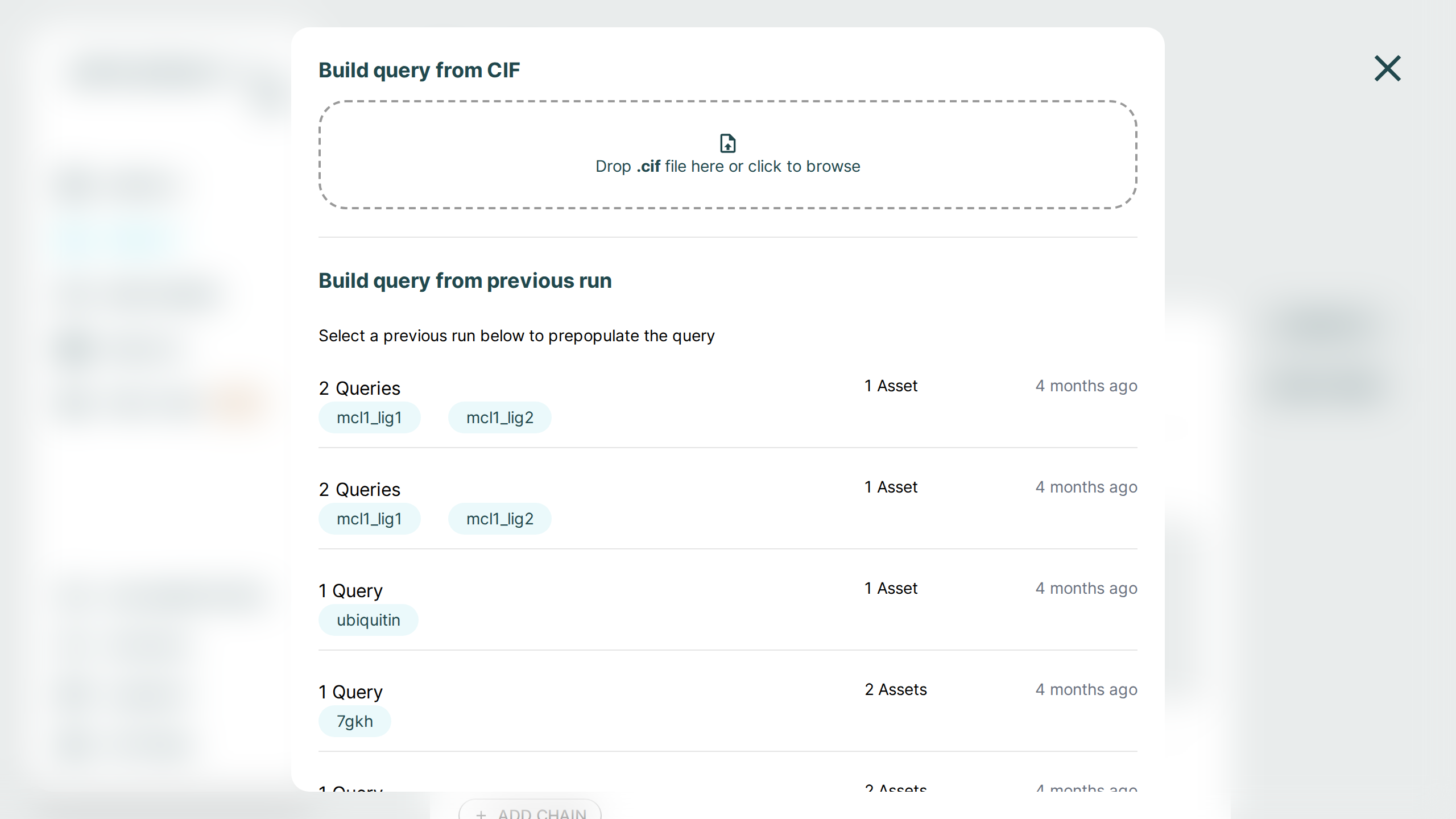
Use the Examples button to load one of the built-in sample queries, or use Start From to initialize a new prediction from either a CIF structure file or from a previous run.
Here are some notable ways to configure a query:
- Molecule Type: Select between Protein, Ligand, RNA, and DNA. There are some type-specific features such as the ability to use SMILES vs CCD code for ligands. You can specify multiple ligands either through separate components with different identifiers, or by separating them with
.as part of one SMILES string, e.g.CCCC.CO. Note that this approach will not result in successful comparisons to attached ground-truth structural data, since this relies on each ligand being assigned a unique chain identifier in both the predicted and attached structures. - Copies: Adjusts the number of copies for the chain. A name is automatically created and usually does not need to be modified. If you'd like to adjust the name, this can be done in the JSON Queries tab.
- Add Chain: Adds a chain to the query. If you need to delete the chain, hover the mouse to the top right. There must always be at least one chain per query.
- Add Query: Add a new query to the request. Hover the mouse to the top right of the query to delete it. Delete will not appear if there is only one query as there must always be at least one query.
JSON Queries Editor🔗
The JSON Queries Editor view is considered an advanced view and it is recommended to instead use the Query Builder to form new queries. The queries made via the Query Builder are reflected in the JSON Editor view but not all changes in the JSON Editor will be reflected back to the Query Builder.
For advanced users, the JSON Editor offers many convenience features such as syntax highlighting, keyword auto-completion, and data type validation.
Tags🔗
Query names that are supplied in the JSON payload are automatically derived as tags for the request. These tags can later be used to search for specific prediction requests.
Custom Tags🔗
You can supply your own tags by typing directly in the "Tags" field. These tags will appear with the results and can be searched for fast lookups across all queries and results. Custom tags are a great way to distinguish between requests that might have similar queries.
Examples🔗
The ApherisFold application comes with examples to help with getting started. Each of these examples can be run across all models. These can be used as starting templates for your queries or as a simple way to evaluate the full workflow.
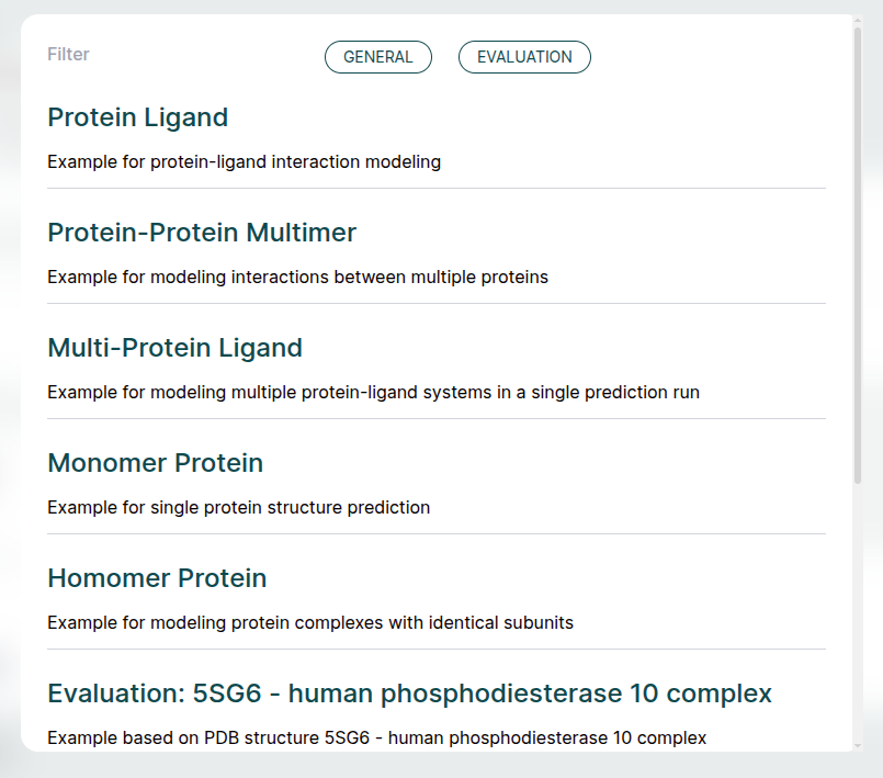
The examples provide MSA files and do not need a MSA server to run. The examples can also be used with configured MSA servers, as described in Multiple Sequence Alignment (MSA).
Below we provide a bit more detail on each example:
- Protein Ligand: The simple use-case of co-folding a small molecule with a single protein chain. The protein chain corresponds to the sequence of MCL1, and the small molecule is Aceclidine.
- Protein-Protein Multimer: Hemoglobin is an example of a query consisting of a multimer of protein chains, with no ligand present.
- Multi-Protein Ligand: A single query consisting of multiple sub-queries. In this case, MCL1 is co-folded with two different ligands (Aceclidine and 1-benzothiophene-2-carboxylic acid).
- Monomer Protein: A single protein chain, Ubiquitin.
- Homomer Protein: A dimer of identical protein chains, in this case the GCN4 Leucine Zipper.
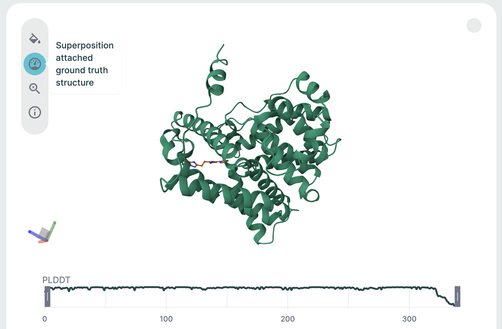
Evaluation Examples🔗
The remaining examples illustrate how the ApherisFold platform can be used to evaluate models on reference structures. Each one is identified by a PDB ID (since the data in these examples is derived from the public domain) and is accompanied by a "{query_name}-ground-truth.cif" file attached as an asset.
Note
If you provide your own .cif files to serve as ground-truth, the name of the file should match the name of the query in your request.
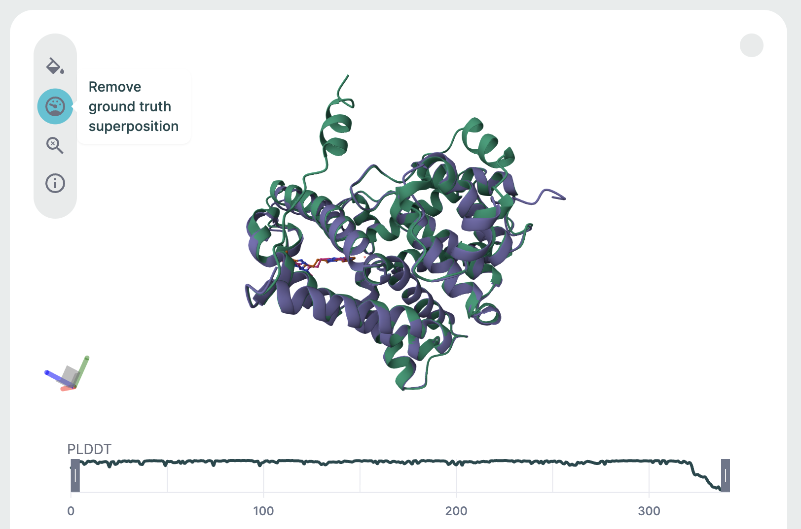
After predicting the structure, the prediction is aligned to this reference structure, and several metrics of structural similarity are computed. The superimposed structures and metrics can then be viewed in the corresponding results page.
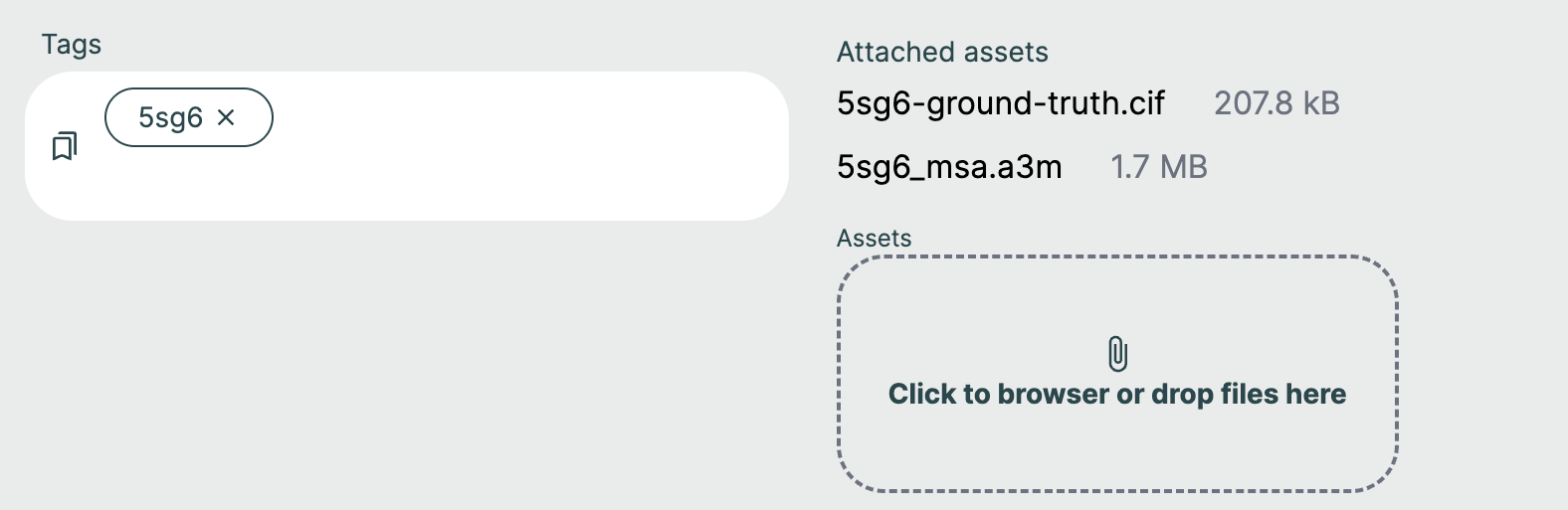
Assets and MSA files🔗
If your request requires additional assets, such as an MSA file, they can be supplied by clicking the Assets button or dropping in files.
Once you have uploaded your assets, they need to be included in your query by clicking the MSA Asset selection dropdown to choose from already added files or upload a new file. The JSON Editor will reflect this with the msa field.
If you want to set your request up as an evaluation of model performance on a known structure, make sure to upload the reference CIF file with the naming schema "{query_name}-ground-truth.cif".
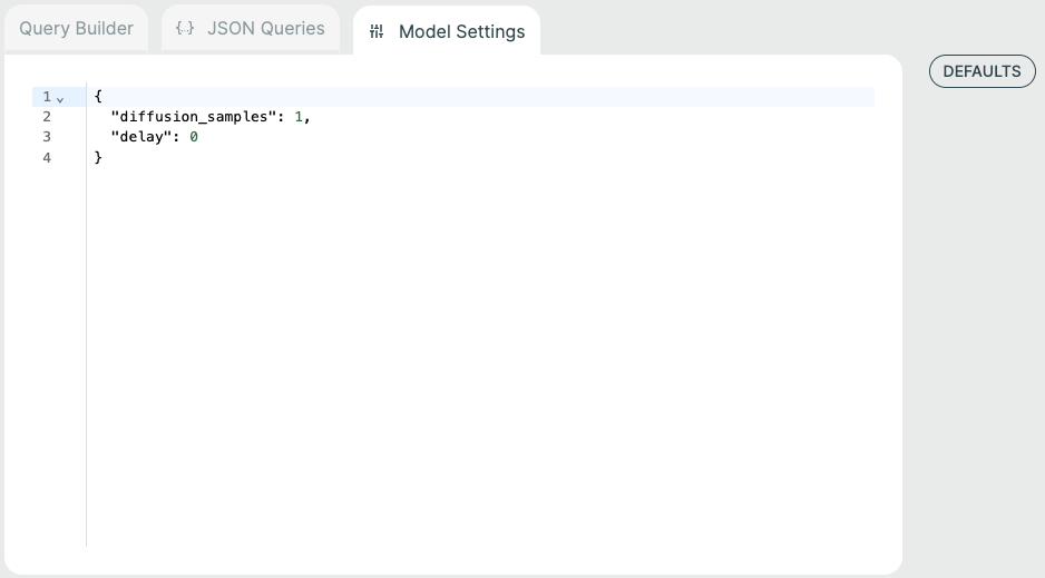
Model Settings🔗
Some models have additional model-specific settings that can be configured such as diffusion samples. These can be changed on the Prediction screen by selecting the "Model Settings" tab at the top.
You can click the "Defaults" button to see the available model settings and make changes.
Results Management🔗
Whatever you submit in the JSON payload (one or multiple queries) is submitted as a single request.
Submitting additional requests will place those requests in a queue. The GPU is fully consumed per request. Parallelism and multi-GPU support will come in follow-up releases.
All submitted requests and results can be viewed on the Results page.
Request Search🔗
You can also filter down results based on tags set for the queries or for metadata such as model name.

Request Status🔗
Submitted requests can have a few statuses:
- Pending
- Running
- Failed
- Cancelled
- Done
- When completed, the status shows the total query runtime.
Queued, pending, and accepted requests display as Pending until they actively start running.
In addition to the request status, you can also see when the request was created, the model and version, and any tags associated with the request.
Reuse a Request in a New Prediction🔗
On any Results detail page, the Job Details section includes a Set up new prediction button. Selecting it opens the Prediction page with the original request pre-populated:
- Request parameters load into the Query Builder and JSON editor in the same format the API expects.
- Tags, model version, and model settings are restored when available.
Within the Predict page, the same workflow is now surfaced under the Start From button. Choosing a previous run there reuses the same saved request details without modifying the original result.
All fields remain editable and submitting creates a brand-new request, leaving the original results unchanged.
Results Deletion🔗
Request results are persisted in the output folder specified when you deployed the Apheris Hub for the first time, either via Docker or Kubernetes.
Currently, there is no built-in way to delete these results. Instead, they are managed through the file system. This is an intentional measure to avoid any accidental deletion of valuable insights.
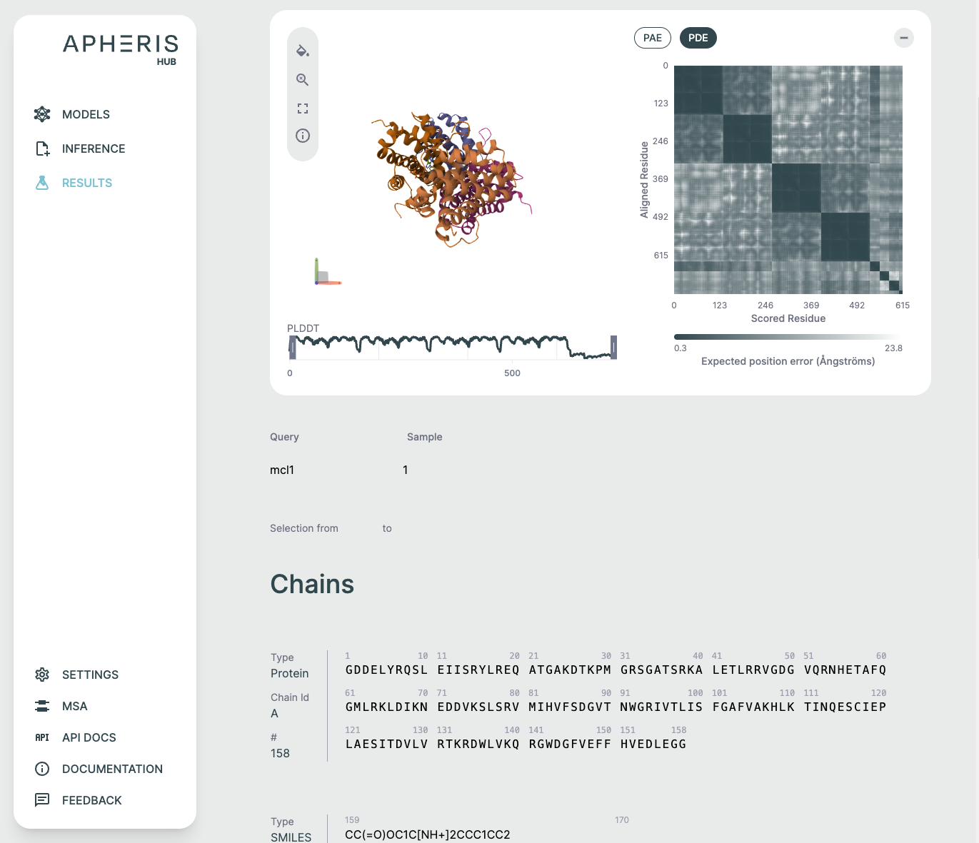
Analyzing Results🔗
The ApherisFold application comes pre-packaged with specialized analysis tools to support analyzing prediction results within the UI.
You can also Download Results by clicking the raw results download button at the top of the results screen.
Each of these visual components serves a specific purpose in interpreting co-folding predictions:
- 3D viewer: Understand overall fold and domain organization
- PAE/PDE: Assess inter-residue or inter-chain confidence
- pLDDT plot: Gauge per-residue reliability
- Sequence section: Review input-output fidelity and interpret ligand participation
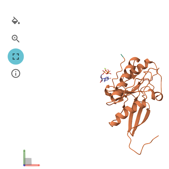
3D Structure Viewer (Left Panel)🔗
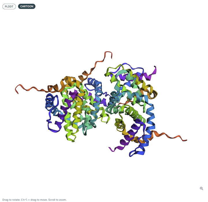
This panel displays the 3D atomic structure of the predicted protein or protein-ligand complex. The cartoon representation emphasizes the secondary structure elements (helices, sheets, loops).
For more details on how to use the 3D Structure Viewer, please see this page. Note that not all of the operations are applicable to ApherisFold.
Viewer Color Coding🔗
The structure is colored based on per-residue pLDDT scores, which indicate the model's confidence in the predicted atomic positions. The scale typically follows:
- Blue: Very high confidence (pLDDT > 90)
- Green: Confident (70–90)
- Yellow/Orange: Low confidence (50–70)
- Red: Very low confidence (< 50)
This can be helpful for visualizing local and global structure quality, identifying disordered or uncertain regions, and verifying expected fold topology.
PAE / PDE Matrix (Right Panel)🔗
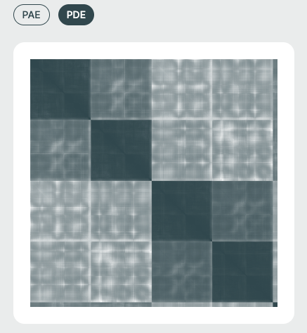
The Predicted Aligned Error (PAE) or Predicted Distance Error (PDE) matrices visualize the model's expected error in positioning residue pairs relative to one another. This is essential for interpreting inter-domain and inter-chain interaction confidence and is especially relevant in multi-chain or protein-ligand complexes.
- PDE: (specific to Boltz-2) is a measure of the uncertainty of the model in the distance between two residues/ligand atoms in the prediction, which is useful for uncertainty-aware modeling.
- PAE: further captures the uncertainty of the model in the relative orientation, in addition to the distance, of pairs of residues/ligand atoms in the prediction. For further reading, there is an excellent visualization created by the European Molecular Biology Laboratory (EMBL) on this guide.
Both of these are most easily visualized as a heat map, where each axis corresponds to sequential Amino Acid/DNA/RNA residues or ligand atoms.
Matrix Color Coding🔗
Darker cells imply lower predicted error (higher confidence), while lighter regions suggest areas of structural uncertainty.
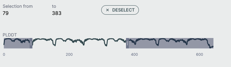
pLDDT Plot🔗
This line graph shows the pLDDT score per residue, providing a quick global overview of prediction confidence. It's ideal for identifying low-confidence loops or disordered regions and useful for downstream filtering (e.g., in docking or dynamics simulations).
- X-axis: Residue index across all chains
- Y-axis: pLDDT score (0–100)
Full-Screen Molecular Viewer🔗
The molecular viewer can be maximized to occupy most of the screen space for detailed structural inspection. In full-screen mode, the 3D viewer, PAE/PDE plot, and sequence bar are displayed together to provide a comprehensive view of the model. Each component can be minimized or expanded individually as needed, while the 3D viewer remains as the main background element for structure visualization.
Chains Sequence Display🔗
This part is helpful for verifying sequence input/output consistency. Ligand info is key for those focused on drug binding or active site modeling.
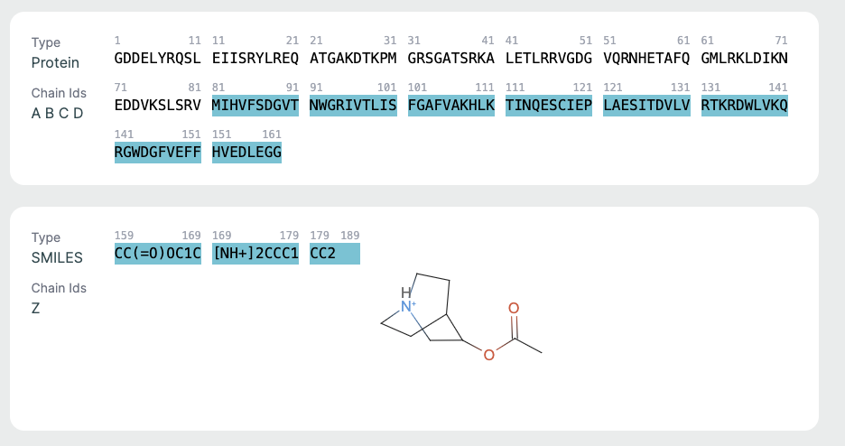
- Displays the full amino acid sequence used for the prediction.
- Includes chain identifiers (A, B, C, etc.).
Ligand Representation (SMILES)🔗
If a ligand is present (as in co-folding), it is shown in SMILES format along with a 2D molecular rendering.
Support and Next Steps🔗
To get access to source code, troubleshoot deployment issues, or inquire about connecting to federated environments, please contact: support@apheris.com.